Optimizing manufacturing production scheduling (MPS) using constraint programming
1. Introduction
Production scheduling primarily deals with arranging different jobs in various machines based on the timelines for each job. There can be numerous combinations of schedules possible. Production schedules can be designed to maximize the capacity utilization, minimize idle time of the machine, earliness, overall costs etc. Manual design of a schedule can be a tedious and time consuming task. There are a lot of dependencies which the scheduler needs to tweak based on a single change. Generating a optimal production schedule targeting a specific objective function can be done using mathematical models.Generating a production schedule targeting a specific objective function can be done using mathematical models. Mathematical models involve formulating the production scheduling problem as an optimization model wherein there is a certain objective function which needs to be optimized based on a set of production constraints. Mathematical models generally outperform manually designed schedules which involve a lot of inter-dependencies among the jobs. Due to improvement in computational power, developing a production schedule using mathematical models is relatively quick and efficient.
We partnered with a client who has multiple manufacturing facilities and requires production schedules for different sites. These production schedules are designed manually keeping in mind fluctuating demand, raw material availability and safety stock requirements. To alter an existing schedule, the schedule planner has to spend countless hours (approx 1-2 days) to make sure all the above requirements are met. Using mathematical models, which act as a production scheduling optimizer , this process can be automated and a schedule can be generated within a few minutes resulting in significant time saving. The requirements for each site were vastly different. Thus, the solution for each site needed to be tailored accordingly to generate the desired outcome.
2. The optimization problem
Optimization deals with finding the best solution among a large set of possible solutions. Following are the common kinds of optimization problems.
- Investment
- Production planning problems and inventory control
- Manpower planning
- Military planning
- Allocation of aircraft to routes
An optimization problem is formulated as a mathematical model that typically consists of an objective function and a set of constraints. The constraints are a set of rules which must be followed. An objective function helps the model to choose the best solution among the possible solutions. The solution from a model can either be feasible, optimal or infeasible. A feasible solution is one which satisfies all the constraints. An optimal solution is one which is feasible and yields the best (maximum or minimum) value of the objective function. Production scheduling methods can be applied to solve optimization problems in production planning, inventory control, and other domains to design schedules that maximize efficiency and minimize cost.
Optimization problems including production scheduling optimization can be solved using the following
- Linear Optimization/Linear Programming
- Linear Programming (LP) involves solving a mathematical problem involving linear objective function and constraints
- LP problems can be solved using graphical methods, simplex methods, branch and bound techniques
- LP problems can also be solved using production scheduling solvers like Glop, SCIP (state of the art algorithms to solve LP problems)
- Constraint Optimization/Constraint Programming
- Constraint Programming (CP) involves finding a set of feasible solutions by using constraints to deduce the values the variables can take. The search space can be narrowed down by taking constraints into account
- CP problem focuses on identifying feasible solutions. CP problems may or may not have an objective function.
- CP problems are solved using CP-SAT solver
2.1. Optimization problem examples
Toy example
Maximize 3x + 4y for the following set of constraints
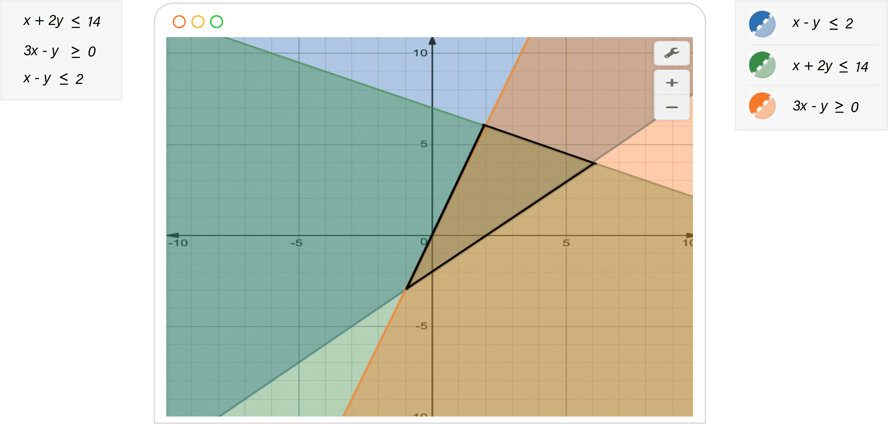
Optimal solution is found by traversing through the boundaries of the feasible region. The optimal solution to the problem is as follows:
x = 6, y = 4, Objective function value = 34
2.2. Job sequencing problem
Problem statement
3 Jobs need to be processed in a single machine. The processing time and the due dates (in days) for each job are given in the following table. The due dates are measured from zero, the assumed start time of the first job.
| Job | Processing time (day) | Due date (day) | Late penalty |
|---|---|---|---|
|
1 |
5 |
25 |
19 |
|
2 |
20 |
22 |
12 |
|
3 |
15 |
35 |
34 |
The objective is to determine the job sequence that minimizes the late penalty for processing all jobs
Definition
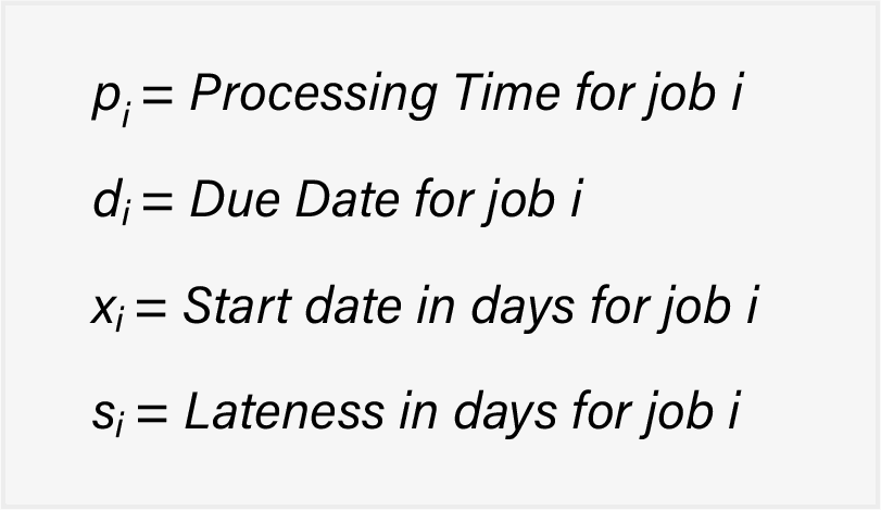
Objective function

Constraints
1. Noninterference/No Overlap Constraints (Two jobs cannot be processed concurrently)
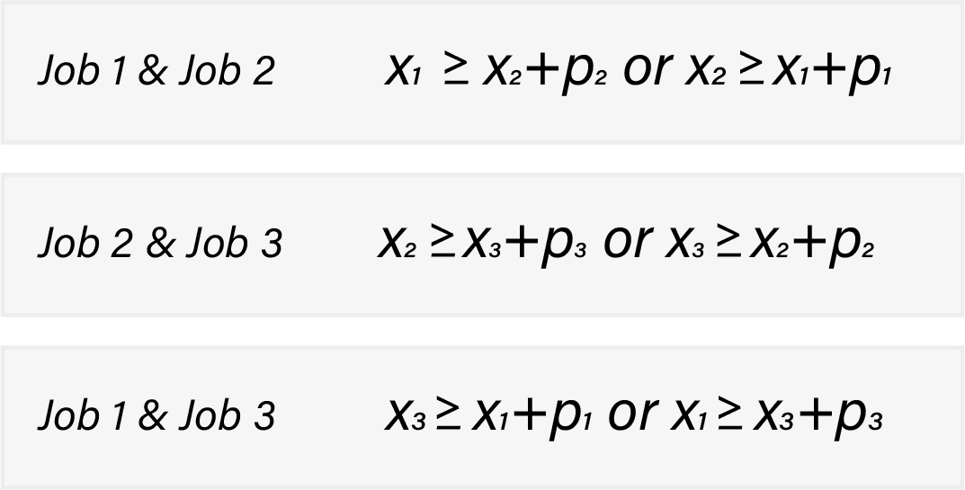
2. Due date constraints

The optimal solution to the problem is as follows:

Job 2 starts at 0, Job 1 starts at 20 and Job 3 starts at 25. The job sequence is 2-1-3. Completion of Job 2, 1 & 3 are 20, 25 and 40 respectively. Job 3 is getting delayed by 5 days.
3. Mathematical models
Production scheduling problems are typically formulated as a mixed integer linear programming (MILP) problem.
3.1. Terminologies in a MILP model

Linear programming refers to an optimization method where the constraints are having linear relationships. The decision variables in MILP can be integer or continuous.
3.2. Job shop scheduling
Job shop scheduling is a form of production scheduling which consists of scheduling of n jobs with varying processing times on several m machines. A job typically consists of a sequence of tasks which need to be performed in a given order and each task must be processed on a specific machine. Job shop scheduling problem is modeled as a MILP problem.
There can be numerous variations of this problem.
- There can be duplicate machines
- A certain gap might be required between jobs
- Machines must run continuously with no idle time
Inputs
The inputs in a job shop problem are described in terms of a recipe. The processing time for each task/stage in a job needs to be specified.
Constraints
The constraints in a job shop problem can be the following.
- No task in a job can be started until the previous task for the same job has been completed
- A machine must have only one task assigned at a time.
- Timelines for a job
- Gap between consecutive tasks in a machine
Objective function
The objective function in a job shop problem can be one of the following
- Minimize makespan (Equivalent to maximizing utilization of machines, Makespan refers to time elapsed between the start date of first job and end date of last job)
- Minimize tardiness
- Minimize production costs
- Multi-objective function
Outputs
Once the model optimizes on a specified objective function, the model spits out the start times for each task for different n jobs. The schedule can be visualized using a Gantt Chart.
4. Production schedules
In the case of the Client, the production schedules were required for two sites namely Site A and Site B. Each site had different processes, constraints and ways of designing the schedule. Batch production was employed in both the sites. Each batch went through various processes/stages until completion. Both the schedules were to be optimized for maximizing the capacity utilization.
Site A – requirements
- Timelines for each batch
- Gap required between the consecutive batch
- Batches must start on particular days of the week
- Batches need to be manufactured in a certain number of clusters
- Schedule needs to be designed for 3 years
Site B – requirements
- Timelines for each batch
- Machine types required for a specific stage – Certain processes in a batch need to be manufactured on a particular machine type. There are a finite number of machines. For a particular batch, only a select few machines can be assigned. The requirement is to choose one machine out of possible ones.
- Schedule needs to be designed for 1 year
- Batches need to be done back to back
- Maximum allowable gap between consecutive batches
For each of the sites, all the above requirements were modeled mathematically in terms of linear relationships to enable production schedule optimization. The primary objective was to achieve high capacity utilization for both the sites. In the optimization model this was achieved by reducing the makespan.
The optimization model generates the sequence of batches and the start and end dates for each process of different batches. This output can be visualized in a Gantt chart.
5. Constraint programming
Constraint programming is an approach similar to mathematical programming which aims to arrive at a solution rapidly given the constraints and objective function. A constraint programming model can provide multiple solutions.
There are several frameworks available for modeling a constraint programming problem. Some of them are Google Optimization Tools (OR-Tools), Pyomo, PuLP and gurobipy (Gurobi Optimization).
OR-Tools is an open source software with excellent documentation and top notch performance. The OR-Tools framework has a solver named CP-SAT Solver which transforms the constraints into clauses and finds values for decision variables. The typical steps in a constraint programming model are as follows.

The CP-SAT Solver is the critical engine for finding solutions to a model. The CP-SAT solver can give a quick feasible solution or optimal solution based on the time limit specified. Finding an optimal solution usually takes longer than a feasible solution. CP-SAT can easily scale for large problems and deduce solutions despite the complexities.
5.1. Site A mathematical model formulation
Problem statement
The sequence in which the batches need to be manufactured are given. The start and end date of each batch need to be determined. The dates are converted to integers. The minimum start date of the schedule is taken as 0.
Objective function
Minimize the gap between the start date and the end date of the first and last batch respectively. Equivalent to maximizing capacity utilization.
Constraints
- Interval for Start date of batch
- Interval for End date of batch
- Relation between Start and End date
- Ensure start date for Product A is particular day
- Gap between consecutive batch
5.2. Site B mathematical model formulation
Problem statement
Each batch goes through various processes/stages during its manufacturing. For each stage, there are specific machines which can be assigned. The scheduling of the batches is dependent on the bottleneck processes. For each batch, once the bottleneck processes are scheduled through optimization, the non-bottleneck process dates can be computed through trivial calculation.
Cell manufacturing is employed at the site. Below figure shows the layout
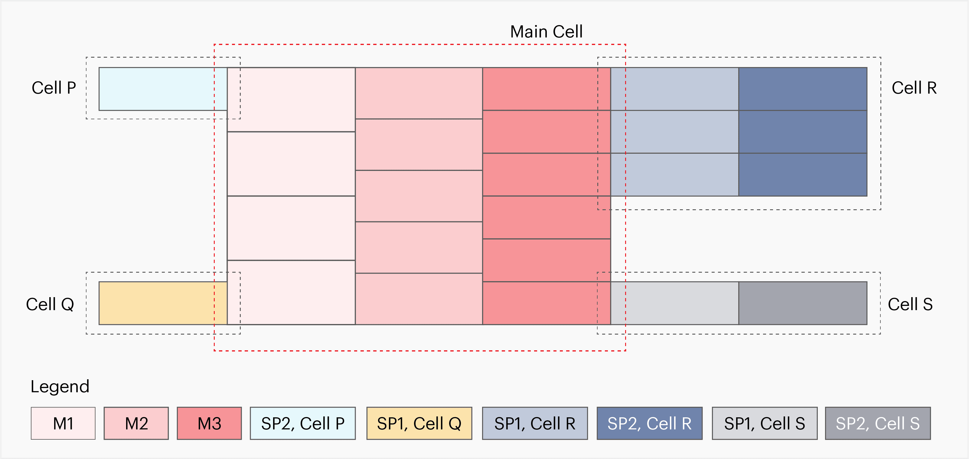
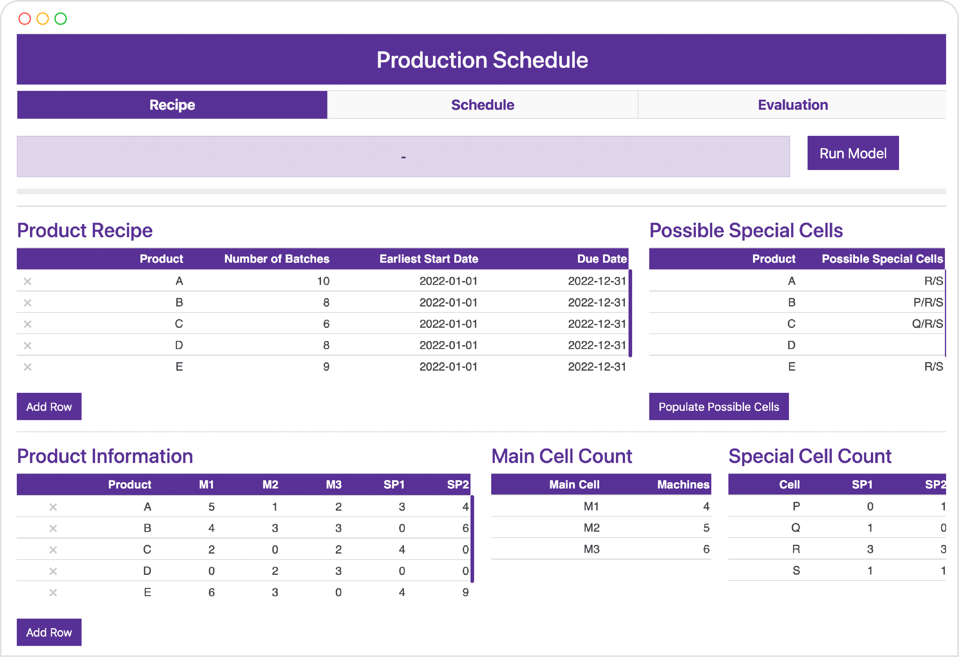
In the main cell, there are three kinds of machine types namely M1, M2 and M3. Apart from the main cell there are 4 special cells namely P, Q, R and S. The special cells contain two types of special purpose machines namely SP1 and SP2. Below table shows the counts of machines in the site.

Each batch goes through the main cell followed by any one of the special cells. Typically the sequence of machine types/processes for a batch is M1, M2, M3, SP1 and SP2. For some batches, some of the machine types in between are not required. There are 4 M1 machines in the Main Cell. Out of 4 any 1 machine would be utilized for processing of the batch. Once a batch is assigned a particular special cell, SP1 and SP2 processing would happen in the same cell. Batches will not move across special cells during their production.
The schedule for this site is divided into two steps. In the first step, for each batch for each process the machine assigned would be deduced. In the second step, the scheduling of the batches would happen. Thus there would be two models namely Machine Assignment Model and Batch Scheduling Model.
Machine assignment model
Objective function
Minimize the sum of error from average duration for each machine type
Constraints
- Constraint to ensure that SP1 and SP2 machines belong to the same cell for each batch
- Constraint to choose one machine for each machine type
- Constraint to ensure that sum of durations is within p and q days of average duration for each machine type
Batch scheduling model
Objective function
Minimize the gap between the start date of the first batch and the end date of the last batch. Equivalent to maximizing capacity utilization.
Constraints
- Interval for Start date of a process in a batch
- Interval for End date of a process in a batch
- Relation between Start and End date
- Relation among process/machine types for a batch
- Start Date of Current Process = End Date of Previous Process
- No Machine Overlap Constraint
Dashboard application for site B
Conclusion
The complexity of production scheduling increases as the number of jobs and machines increase. Mathematical models are able to solve such problems taking into account the set requirements and goals with tremendous ease, speed, and accuracy. This has significant business impact in terms of reducing the countless hours spent on editing a manually created schedule to meet the requirements.
Talk to our expert
Let’s discuss how you can leverage our Data Science services to identify business problems and enable business transformation.
About the author
Akshay Matam is an Associate Lead Data Scientist with 5 years of Machine Learning and Data Science experience. He has worked in building Optimisation models, Natural Language Processing tools, Data Analysis and Insights delivery. He has experience in working with pharma and cpg clients.
Nitish Sawant is a Data Scientist at Sigmoid with a background in Industrial Engineering. He has solved problems involving optimisation and semantic search in NLP. He has expertise working across various ML algorithms and deep learning techniques.


