How to optimize Nested Queries using Apache Spark
Reading Time: 9 minutes

Spark has a great query optimization capability that can significantly improve the execution time of queries and ensure cost reduction. However, when it comes to nested queries, there is a need to further advanced spark optimization techniques. Nested queries typically include multiple dimensions and metrics such as “OR” and “AND” operations along with millions of values that need to be filtered out.
For instance, when Spark is executed with a query of, say 100 filters, with nested operations between them, the execution process slows down. Since there are multiple dimensions involved, it takes a huge amount of time for the optimization process. Depending upon the cluster size, it may take hours to process Apache Spark DataFrames with those filters.
In this blog, we will walk you through common challenges faced while working with nested filter queries and we were able to optimize query using logical tree optimization. We found that upon tweaking some of the codes and applying a common algorithm, we were able to reduce the total cost and execution time of the query.
We could further optimize the logical plan and send processed data to apply filters, thus reducing the total load on processing. The logical query is optimized in such a way that there’s always a predicate pushdown for optimal execution of the next part of the query. We used Apache Spark with scala API for this use case.
Problem Statement
The user needed to filter out all values from the millions of single columns of records from a file. For this filter file, the supported filters are “include” and “exclude”. The user can select multiple dimensions for applying filters and can combine them with a filter operator which is either “AND” or “OR” or both. So, the user could now create a nested filter expression containing multiple dimensions with both “OR” and “AND” operations between them.
This requirement was to be implemented in our product SigView. For this use case, we developed a feature called Bulk Filter (as it includes “OR” operation between filter dimensions). All the filters inside the Bulk Filter are rearranged on the basis of cost, forming an optimized group of filters for processing.
Optimization Plan Description
- Filter Expression
- Each filter expression is a tree that is composed of nodes
- Each node is immutable and consists of either:
- Filter expression having dimensions and values with filter operations called filter nodes
- Or combinations of filter nodes with an operator to be applied between them (operator is either “OR” or “AND”) called nested nodes
- Filter nodes are called as ProjectionBulkFilter class
- Nested Nodes are called the BulkFilter class
- Optimization Rules
- Every node needs to be executed
- Hence, the fewer nodes we have, the faster the execution
- Each node will have a df(DataFrame) passed for processing
- More the size of df, slower the execution
- If a filter is applied on df and there is some amount of predicate pushdown on preprocessing of that df, the size of the df can be minimized which is to be passed to the next node, thus decreasing the total execution time
- In a nested query, where each node is nested together with an operator, the nodes can be distributed on the basis of the predicate pushdown. Thus, calculating the cost for each node’s execution and re-arranging in an increasing order of cost. And executing on the same calculated order
- This reduces the load on each node, where filtered/processed df is passed after each execution.Thus, maintaining a predicate pushdown with optimizing the logical plan for faster execution
- Defining operator coefficients
- Lemma
- Let us assume that each joins with a filter result in 10% of base data size (90% data is filtered out) (here for filtering millions of values join is used)
- A union is “Union ALL” in Spark that basically combines together rows of two source DataFrames
- Based on the above tenets we are defining the following three coefficients
- Cost coefficient of each filter Join operation = 0.1
- AND: multiply(children) i.e. Multiplication of cost of each child BulkFilter instance
- OR: sum(children) * 10 i.e Sum of cost of each child BulkFilter instance * 10
- Illustration: For the following Bulk Filter Expressions, the Cost Calculations are below:
a and (b or c) and (d and e) -
- AND
- a = 0.10
- OR =2 (0.20 * 10)
- b = 0.1
- c = 0.1
- AND = 0.01
- d = 0.1
- e = 0.1
- AND
- a and (b or c) and (d and e) and (x and (w or y))
-
- a = 0.10
- OR =2 (0.20 * 10)
- b = 0.1
- c = 0.1
- Lemma
Implementation Approach
- Rearrange the BulkFilter(BF) object’s instances on the basis of cost
- Low-cost instances should be on the left side
- High cost should be on the right side
- This is a type of predicate pushdown, where we are pushing smaller instances before the larger instances so that the larger instances will have fewer data to read on
- This will be done to all nested instances
- For eg: we have BF as
- (a or b) and c and (d or f)
- Since there are two instances of BF and 1 ProjectionBulkFilter(PBF)
- As the operator between them is “AND”, we need to re-arrange the instances on the basis of cost
- so the arranged form will be:
- c and (a or b) and (d or f)
- We are arranging them so that the less costly will be processed first and their output will be input for the next instance
- In the above case, after arranging, c will be executed then it’s output will be sent to the next instance (a or b) as input df and similarly
- Assign the operator coefficients for each operator, which is used to calculate the cost of each BulkFilter node
- The cost will be on the basis of no. of nodes and the operator coefficients
- Decide the input for the next instance on the basis of operator
- On the basis of the operator decide the input for the next instance
- In the case of “OR”, we have to send the baseDF to all instances
- In the case of “And”, we need to send the processed df to the next instance
- For eg: we have below case
- c and (a or b) and (d or f)
- As the operator is “AND” between them, the c should be processed first
- Then it’s output is sent to (a or b) for processing a,b and (a or b)
- Now, after (a or b) is processed, the output of (a or b) will be sent to (d or f)
- The output of (d or f) will be the output for the above instance
- c or (a or b) or (d or f)
- The baseDF is passed to each instance as input and is reduced with OR between them
- c and (a or b) and (d or f)
Class Creation
- Data Type
- Filter Expression
- Filter nodes are called as ProjectionBulkFilter class.
- Nested Nodes are called the BulkFilter class.
- Classes and Object
- Scala Class for Filter expressions
- case class ProjectionBulkFilter(key: Column,fileLocation: String,operation: String) – PBF
- It’s the lowest level of Filter Expression. The supported operations are:
- Include – Inner Join
- Exclude – Anti-left
- It’s the lowest level of Filter Expression. The supported operations are:
- case class BulkFilter(operator: String, instance : List[Either[ProjectionBulkFilter, BulkFilter]]) – BF
- It contains an operator and a list of either ProjectionBulkFilter or Itself
- The supported operator are: AND & OR
- case class ProjectionBulkFilter(key: Column,fileLocation: String,operation: String) – PBF
- Helper classes for calculating cost, and sorting on the basis of it
- case class ProjectionBulkFilterWithPoints(key: Column,fileLocation: String,operation: String,points:Double) – PBFWP
- It’s similar to ProjectionBulkFilter except it contains an extra class variable point which is the cost of it
- case class BulkFilterWithPoints(operator: String, instance : List[Any],points:Double) – BFWP
- It’s similar to BulkFilter except it contains an extra class variable point which is the cost of it
- Scala Class for Filter expressions
Implementation Strategies
- Getting cost for BF
- Strategies: bottom-up and level-order
- If it’s a PBF, return PBFWP with 0.1 points
- If it’s a PBF, return PBFWP with 0.1 points
- If it’s a BF
- Recursively run this method for BF
- Return a BFWP with points, which is the output from below “reduce” method
- If it’s a PBF, return PBFWP with 0.1 points
- Strategies: bottom-up and level-order
- Reduce method to get points of each BF
- Traverse through the instance of the BF
- If it’s a PBF, return 0.1.
- If it’s a BF, return reduce(BF)
- After assigning the points, reduce by operator coefficients:
- If “OR” : (sum of the cost of all level nodes) *10
- If “AND” : (product of the cost of each node in the same level)
- Sort on the basis of Cost
- Strategies: Bottom-up and level-order
- After assigning cost for each node, traverse through the node and apply sortBy for its instance(level)
- The sortBy has points as key to sort
- Whichever node on the same level has the lowest points will be on the left side and the node having the highest points will be on the right side (sorted in ascending order)
- The sort occurs for each nested instance of BF
- When all levels are sorted from bottom-up, the top level is again sorted in a similar way
- Strategies: Bottom-up and level-order
- Applying and reducing BF
- Strategies: Bottom-up and level-order
- Traverse through the graph and for each node do as below
- If the node is a PBFWP, reduce it by applying applyBulkFilterForEachDimension method
- If the operator for this level is And, pass the output of this node to the next node as an input DataFrame
- If the node is a BFWP, reduce recursively for its child nodes.
- If the operator for this level is And, pass the output of this node to the next node as the input DataFrame
- Finally, reduce on the basis of the operator:
- If the operator is OR: apply Union and dropDuplicates on all data frames reduced from its child nodes
- If the operator is And: return the last df on the reduced list of DF
- Strategies: Bottom-up and level-order
Illustrations
- Getting cost for BF
- Suppose we have a DataFrame for cars called carDF
- And have four filters A,B,C and D as:
- A -> cars of color (green,blue,white,grey,silver,gold,yellow)
- B -> cars of color (blue,green,silver)
- C -> cars of brand (BMW,Hyundia,Tata)
- D -> cars of region (ASIA,NA,EUROPE)
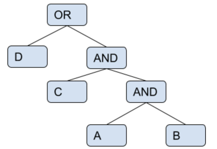
- And have nested query as:
- (D) or ((C) and (A and B))
- The Parse tree will be as :
- So, if we apply a filter in baseDF “carDF” without predicate pushdown, the carDF will be passed as input df to all leaf nodes/filters. As shown below:
- (carDF ^ D) OR ((carDF^C) AND ((carDF^A) AND (carDF^B)))
- Here, ^ : stands denotes filter
- As we can see from above, there’s a chance of optimization for each leaf, if the operator is “AND” we can pass processed df as an input to the next leaf, else the baseDF if the operator is “OR”
- So, for the above case if we apply the given algorithm and cost optimization, the nested query will be changed as:
- (((A and B) and C) or D)
- Now, A and B can be processed and its output can be passed as input to C
- As, if we visualize the tree there are two nodes from the parent, to which baseDF can be passed as input
- So, for D filter operation will be -> carDF ^ D
- For ((A and B) and C), the baseDF will be passed to its child as input, for the operator is “AND”, until we get a leaf node.
- Now, A will be processed -> carDF ^ A = carDFfa (filtered with A)
- carDFfa will be passed as input to B -> carDFfa ^ B = carDFfab
- carDFfab will be passed as input to C -> carDFfab ^ C = carDFfabc
- So, as we can see some predicate pushdown where only a portion of baseDF is passed for filters thus reducing the total load on execution
- So, the output for the whole tree will be :
- carDFfabc OR D -> (carDFabc union (carDF ^ D) = carDFabcd (union as operator is OR)
- Suppose, we have nested query as :
- ((B OR C) AND A)
- After, optimization the query will be changed to :
- ((A) and (B or C))
- The tree will be:

- So, baseDF will be passed to A. So the output will: carDF ^ A -> carDFfa
- As, operator between (A) and (B OR C) is “AND”, So the output of A will be passed as input to the tree (B OR C). Thus, reducing the total size of data to be processed for the next node
- So, carDFfa is passed to both leaf nodes of B and C as input DF
Conclusion
By implementing above strategies, we could optimize the logical plan of the nested query. This technique rearranges the filter expressions in an optimized logical query applying all predicate pushdown, thus decreasing the total execution time and cost of execution. Using this approach, the nested queries are processed faster while taking less computation time and resources.
About the Author
Pravin Mehta is a Data Engineer at Sigmoid. He is passionate about solving problems using big data technologies,open source and cloud services, and he has keen interest in Apache spark and its optimization.
Featured blogs


Featured blogs